Roofline Performance Model
Performance models and tools are an integral part of the performance analysis and performance optimization process for users who seek higher performance and better utilization of the hardware. The Roofline performance model offers an intuitive and insightful way to compare application performance against machine capabilities, track progress towards optimality, and identify bottlenecks, inefficiencies, and limitations in software implementations and architecture designs. Its ability to extract key computational characteristics and abstract away the complexity of modern memory hierarchies has made Roofline-based analysis an increasingly popular tool in the HPC community.
Roofline Performance Model
The most standard Roofline model is as follows. It can be used to bound floating-point performance (GFLOP/s) as a function of machine peak performance, machine peak bandwidth, and arithmetic intensity of the application. The resultant curve (hollow purple) can be viewed as a performance envelope under which kernel or application performance exists.
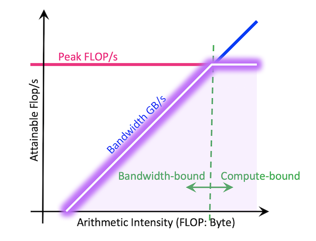
The ridge point on the Roofline is called the 'machine balance' point. Usually, if an application's arithmetic intensity is lower than this point, it is considered to be bandwidth bound, i.e., bound by how fast the data can be moved through the memory system instead of how fast the calculations can be done on the CPU core or the GPU SMs. To optimize in this case, memory inefficiencies are usually good places to examine, such as the memory access pattern, data locality and cache reuse. On the other hand, if the application's arithmetic intensity is higher than machine balance, then the application is more likely to be limited by how fast the computation can be done. In this case, improving vectorization (to more efficiently utilize the vector units on each CPU core), or multi-threading (to utilize the multi or many cores better), can usually help.
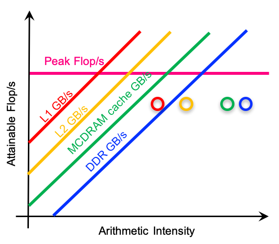
To help look into the complex memory system on modern architectures, multiple Rooflines can be superimposed upon each other to represent different cache levels in the memory hierarchy, and this is called the hierarchical Roofline model. It helps analyze the application's data locality and cache reuse pattern, and understand how efficiently data is flowing through the memory system. A demonstration of a hierarchical Roofline chart is as follows.
To construct an accurate and meaningful Roofline, we will need to collect performance information such as the peak compute performance and peak bandwidth for the architecture, and arithmetic intensity and achieved throughput (FLOP/s) for the application. In the following, we will detail how to collect such information using various performance tools.
Empirical Roofline Toolkit (ERT) for machine characterization
To estimate the peak compute performance (FLOP/s) and peak bandwidth, vendor specifications can be a good starting point. They give insight into the scale of the machine's capabilities, however they may not capture the realistic execution environment that actual applications run in, such as the power/energy constraints and programming models used. To get a more accurate understanding of the machine's attainable peak, the Empirical Roofline Toolkit (ERT) is recommended. ERT runs a variety of micro-kernels and sweeps through a range of runtime configurations. These micro-kernels may be small and designed to just test a particular aspect of the system, but together they provide a more realistic set of estimations for the machine capability such as peak bandwidth on various cache levels, and peak GFLOP/s.
Arithmetic Intensity (AI) and achieved performance (FLOP/s)
To characterize an application on a Roofline, three pieces of information need to be collected about the application: run time, total number of FLOPs performed, and the total number of bytes moved (both read and written). This can be for the entire application or for only a code region that is of interest. For hierarchical Roofline, multiple bytes values will need to be collected for different memory/cache levels, as can be seen in the hierarchical Roofline above (same kernel has different bytes values and different arithmetic intensities on different levels of cache).
For large-scale applications, it is infeasible to estimate the FLOPs or bytes by hand and performance tools are recommended. With recent years' collaboration with Intel and NVIDIA, automated Roofline data collection has been implemented in Nsight Compute. These tools provide fully integrated, production-quality Roofline analysis features and should be the go-to tools; however for completeness, we document a few alternatives, for users who seek lighter-weight tools or more customized data collection workflows. We will focus on the NVIDIA V100 GPU architecture, and the tools discussed will be nvprof and Nsight Compute.
As of mid-2020, the Roofline analysis feature shipped in Nsight Compute by default is only for the device memory (or HBM) level Roofline analysis. However, it can be extended to a hierarchical Roofline using the customized Nsight Compute section files, or Nsight Compute metrics-based data collection methodologies, documented here: the Roofline on NVIDIA GPUs repository.
Arithmetic Intensity
Arithmetic Intensity (AI) is the ratio of total floating-point operations (FLOPs) performed by a given code or code section, to the total data movement (Bytes) required to support those FLOPs. Here please note the difference between FLOPs and FLOP/s, where FLOPs is the count and FLOP/s is the rate or throughput. As mentioned above, for hierarchical Roofline, different 'bytes' will be collected for different levels of cache. For example, the L2 level Roofline will use the 'bytes' for between L2 and L1, and this 'bytes' will be used as the denominator for the L2 arithmetic intensity as well.
Arithmetic Intensity (AI) on V100
NVIDIA's profiling tool nvprof and Nsight Compute can be used to measure FLOPs and Bytes on an NVIDIA GPU. For example, the following command line can be used to collect such information with nvprof, for a particular invocation of a particular kernel in a GPU code.
nvprof --kernels "{kernel name}, {[context id/name]:[stream id/name]:[kernel name]:[invocation]}" --metrics flop_count_dp --metrics dram_read_transactions --metrics dram_write_transactions foo.exe
where flop_count_dp is the total FLOP count for FP64 operations, and dram_read_transactions and dram_write_transactions are the read and write transactions from and to HBM. For FP32 or FP16 operations, flop_count_sp and flop_count_hp can be used. The size of each memory transaction is 32 bytes, so the total HBM data movement can be calculated as (dram_read_transactions + dram_write_transactions) x 32B.
The arithmetic intensity of a kernel on an NVIDIA V100 can then be calculated as,
AI (HBM) = flop_count_dp / ((dram_read_transactions + dram_write_transactions)*32)
For more details on the nvprof or Nsight Compute metrics for hierarchical Roofline data collection, please see the Roofline on NVIDIA GPUs repository and the Hierarchical Roofline Analysis: How to Collect Data using Performance Tools on Intel CPUs and NVIDIA GPUs paper.
Application Performance
The y-coordinate of a kernel on the Roofline chart is its sustained computational throughput (GFLOP/s), and this can be calculated as FLOPs / Runtime. The Runtime can be obtained by timers in the code and the FLOPs from the nvprof or Nsight Compute tool.
Together with the arithmetic intensity (obtained from the previous section) and Roofline ceilings (obtained from ERT), we can then construct a Roofline chart.
Some example scripts are available at https://github.com/cyanguwa/nersc-roofline, demonstrating how an example code from BerkeleyGW, called General Plasmon Pole (GPP), can be modeled by Roofline on both Intel KNL and NVIDIA V100. The paper Hierarchical Roofline Analysis: How to Collect Data using Performance Tools on Intel CPUs and NVIDIA GPUs accompanies these scripts.
With GPP, as we artificially increase the number of iterations for the innermost loop nw from 1 to 6, we get the following Roofline chart on NVIDIA V100 (this is only for HBM level Roofline).
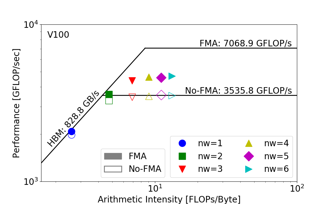
As you can see, as the parameter nw increases from 1 to 6, so does the arithmetic intensity of the application, because the total amount of data moved isn't changed but the total amount of FLOPs executed has been proportionally growing to the value of nw. This increase in arithmetic intensity takes GPP from a bandwidth bound regime to a compute bound regime, and the observed GFLOP/s also increases on the V100 Roofline. The subtlety here is that the bottleneck may be different even for the same nw. For example, at nw=2, the kernel is more compute bound on the V100, where it may be more bandwidth bound on other architectures.
Roofline is able to capture these subtle differences and is very helpful in understanding an application's performance across multiple architectures.