TomoPy
Overview
This case study presents the migration of TomoPy (Tomographic Reconstruction in Python) to the GPU. TomoPy has achieved performance improvements exceeding 500x on the GPU per-slice and greater than 150x on a full dataset for NVIDIA A100s relative to the Edison supercomputer.
Single Slice Results
| Algorithm | Filename | Cores | Iterations | Dimensions | Time to Solution (sec) | |
|---|---|---|---|---|---|---|
| Edison | sirt | tomo_0001 | 1 | 100 | 2048 x 2048 | 28069 |
| Edison | mlem | 28733 | ||||
| Perlmutter | sirt (NN) | 4 | 57 | |||
| Perlmutter | mlem (NN) | 57 |
24 Slice Results
| Algorithm | Filename | Cores | Iterations | Dimensions | Time to Solution (sec) | |
|---|---|---|---|---|---|---|
| Edison | sirt | tomo_0001 | 48 | 100 | 2048 x 2048 | 28069 |
| Edison | mlem | 28733 | ||||
| Perlmutter | sirt (NN) | 64 | 177 | |||
| Perlmutter | mlem (NN) | 178 |
Background
Tomographic reconstruction creates three-dimensional views of an object by combining two-dimensional images taken from multiple directions, for example, this is how a CAT (computer-aided tomography) scanner generates 3D views of the heart or brain.
Data collection can be rapid, but the required computations are massive and often the beamline staff can be overwhelmed by data that are collected far faster than corrections and reconstruction can be performed. Further, many common experimental perturbations can degrade the quality of tomographs, unless corrections are applied.
To address the needs for image correction and tomographic reconstruction in an instrument independent manner, the TomoPy (Tomographic Reconstruction in Python) code was developed, which is a parallelizable high performance reconstruction code.
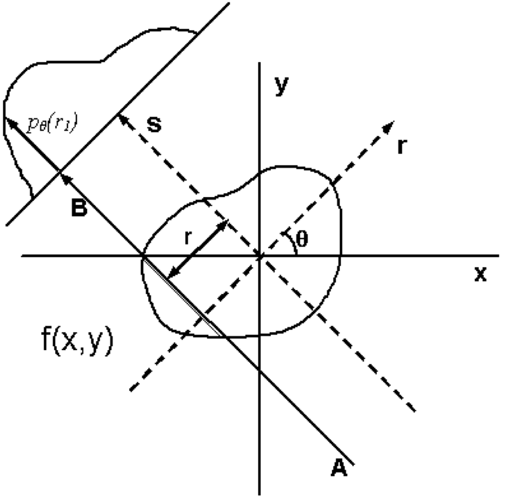
In general, a reconstruction starts with an array of projection angles and the array of projection values at each projection angle and simulates the imaging in reverse.
At the given projection angle in the given slice, there is a detector pixel value whose value represents the attenuation through the medium. The array of these pixels form the projection matrix. If this attenuation measurement is recorded at enough different angles, one can reconstruct an image representing the density of the object.
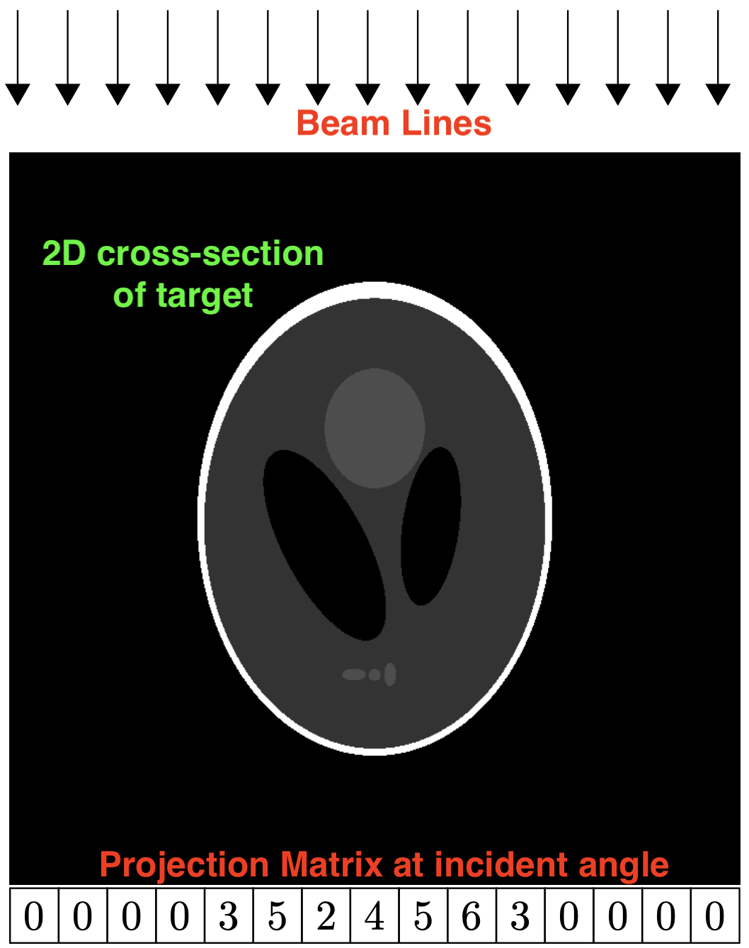
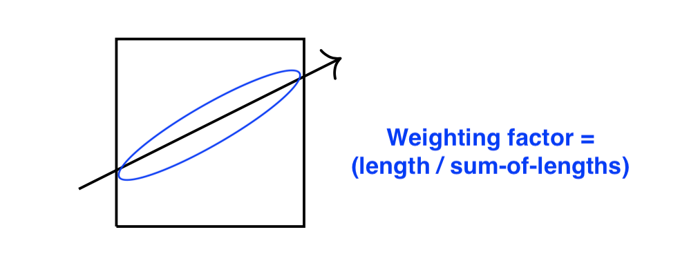
During reconstruction, the beam lines are back-propagated through the reconstruction array for all the known projection angles. During this back-propagation, the traversal distance and offset from the center of the beam line through each pixels in the reconstruction array are calculated. The value of the projection matrix is then "distributed" along all the intersecting pixels according to the calculated weighting factor: (chord-length-through-pixel) / (sum-of-all-chord-lengths):
Original Software Characteristics
The starting point of this case study was 4 years into TomoPy's lifetime (v1.1). The coding model was a thin "glue" layer of Python that provided access to efficient code written in C. The parallelism was implemented at the Python level -- a pool of threads were started using the multiprocessing module and the number of slices were divided among the threads. The performance characteristics were perfect strong-scaling for each slice being reconstructed. In other words, with 4 cores, 4 slices could be reconstructed in the same amount of time as 1 core and 1 slice. However, there was zero weak scaling: parallelism was restricted to the slice level and there were zero performance benefits once the number of threads exceeded the number of slices.
From a high-level point of view, iterative tomographic reconstruction contains a series of nested loops:
// number of iterations               # 1 - 500+
for(i = 0; i < num_iter; i++)
    // the number of slices           # 1 - 500+
    for(s = 0; s < dy; s++)
        // the projection angles      # 360 - 1500+
        for(p = 0; p < dt; p++)
            // the detector pixels    # 512 - 2048+
            for(d = 0; d < dx; d++)
            {
                // ...
            }
The original implementation allocated all the necessary memory outside of all the loops:
// arrays of intersection points
float* ax     = (float*) malloc((ngridx + ngridy) * sizeof(float));
float* ay     = (float*) malloc((ngridx + ngridy) * sizeof(float));
float* bx     = (float*) malloc((ngridx + ngridy) * sizeof(float));
float* by     = (float*) malloc((ngridx + ngridy) * sizeof(float));
// sorted intersection points
float* coorx  = (float*) malloc((ngridx + ngridy) * sizeof(float));
float* coory  = (float*) malloc((ngridx + ngridy) * sizeof(float));
// distances between intersection points and index mapping
float* dist   = (float*) malloc((ngridx + ngridy) * sizeof(float));
int*   indi   = (int*)   malloc((ngridx + ngridy) * sizeof(int));

// number of iterations               # 1 - 500+
for(i = 0; i < num_iter; i++)
    // the number of slices           # 1 - 500+
    for(s = 0; s < dy; s++)
    {
        // ...
    }
The content of the innermost loop was a series of function calls:
- Calculate the intersection coordinates
- Trim the intersection coordinates
- Sort the intersection coordinates
- Calculate the intersection distances
- Calculate the weighting factor
- Distribute the projection matrix values to pixels according to weighting factor
Migrating to the GPU
The initial implementation was a straight-forward translation of the original workflow to the GPU, i.e. the 6 functions in the innermost loop were converted to CUDA kernels.
Common optimizations were implemented:
- Minimize data transfers
- Introduced streams
- Block and grid size optimizations
CUDA streams were utilized in the projection angle loop and synchronized when the reconstruction slice was updated, e.g.:
std::array<cudaStream_t, 8> streams{};
// ... initialize streams ...

for(i = 0; i < num_iter; i++)
    for(s = 0; s < dy; s++)         // slices
    {
        for(p = 0; p < dt; p++)     // projection angles
        {
            auto stream = streams[d % streams.size()];
            for(d = 0; d < dx; d++) // pixels
            {
                // ...
                calc_coords<<<..., stream>>>(...);
                // ...
            }
        }
        // sync all streams
        for(auto itr : streams)
            cudaStreamSynchronize(itr);
        // ... update reconstruction array ...
    }
Significant progress was achieved with respect to the original GPU implementation but the end result was still slightly slower than CPU. "Sorting" and "trimming" were significant bottlenecks and consumed 95% of run-time. Furthermore, the implementation had other issues: it required a very large number of kernel launches -- in a realistic reconstruction, 18,420,000 kernels were launched for each slice1 -- and memory access was inherently strided in a main kernel:
for(int n = 0; n < size; ++n)
    simdata[i] += model[indi[n] + j] * dist[n];
Given the relatively similar compute times on CPU vs. GPU, a secondary thread-pool was introduced per "Python" thread to handle large data sets with 1,000+ slices. The idea was to increase parallelism and further sub-divide the work between the CPU and GPU, i.e. use GPU to supplement CPU when exceeding the number of available CPU cores and if GPU began to out-perform CPU, offload to GPU until OOM and the threads would fall back to CPU.
Ultimately though, it was realized that we were attempting to optimize an algorithm which was designed for CPUs and new approach was required to obtain any notable speed-up.
Developing Rotation-based Reconstruction on the GPU
During a meeting with the tomopy PI, he noted there was a rotation-based technique no longer used in tomography (for performance reasons) that removed the sorting and trimming requirements and where all the weight factors became 1. The reason the algorithm was no longer used was because it was much more computationally expensive:
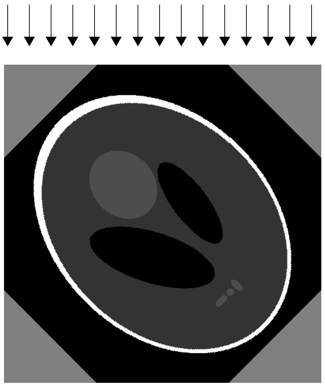
- Rotated the entire region of interest (ROI) to be parallel with the incident ray
- Instead of "rotating" the incident ray
- Interpolated the pixels to their new coordinates
- Required padding the projection to account for pixel loss during rotation
Furthermore, in addition to removing the sorting and trimming bottlenecks, the method also aligned the memory access. In other words, there was an alternative algorithm which was more computationally expensive and increased the problem size but removed our parallelism bottlenecks:
The new algorithm essentially turned the per-projection workflow into:
- Rotate ROI by −θ
- Distribute projection value along a row of pixel values in ROI
- Rotate ROI by +θ
- Update reconstruction
For the rotation of the ROI, we utilized NVIDIA Performance Primitives (NPP) library and re-ordered the loops so that NPP was saturated with independent per-slice rotations:
for(int p = 0; p < dt; ++p)     // projection angles
    for(int s = 0; s < dy; ++s) // slices
    {
        auto* _update = update + (s * nx * ny);
        auto* _recon  = recon  + (s * nx * ny);
        auto* _rot    = rot    + (s * nx * ny);
        auto* _tmp    = tmp    + (s * nx * ny);
        auto* _data   = data   + (s * dt * dx);

        // forward-rotate
        nppiRotate_32f_C1R(_rot, _recon, -theta_p, ...);

        // compute simdata
        pixels_kernel<<<...>>>(..., _rot, _data);

        // back-rotate
        nppiRotate_32f_C1R(_tmp, _rot, theta_p, ...);

        // update shared update array
        atomic_add<<<...>>>(_update, _tmp, ...);
    }
The result of this algorithm changed culminated in the results provided in the Single Slice Results Section and 24 Slice Results Section.
Notes About NPP Usage
NPP does not support multiple GPUs within the same process. Thus, in order to leverage multiple GPUs, tomopy replaced its usage of a thread pool at the python level with a process pool when the GPU-accelerated backend is requested. Furthermore, in order to use streams, NPP requires a call to nppSetStream(...) before subsequent calls to algorithms such as nppiRotate_32f_C1R as opposed to nppiRotate_32f_C1R accepting an additional cudaStream_t argument. This design caused issues for the secondary thread-pool within tomopy (implemented in C++ with a tasking library) which parallelizes the loop over the slices since each thread must refrain from calling nppSetStream while another thread is in-between it calling nppSetStream and calling it's subsequent nppiRotate_* function. The solutions for these problems have been provided below.
Original Tomopy Thread Pool Implementation
def _dist_recon(tomo, center, recon, algorithm, args, kwargs, ncore, nchunk):

    # ...
    with cf.ThreadPoolExecutor(ncore) as e:
        for slc in use_slcs:
            e.submit(algorithm, tomo[slc], center[slc], recon[slc], *args, **kwargs)
Tomopy Process Pool Implementation for CUDA
def _run_accel_algorithm(idx, _func, tomo, center, recon, *_args, **_kwargs):
    # set the device to the specified index within the new process
    os.environ["TOMOPY_DEVICE_NUM"] = "{}".format(idx)
    # execute the accelerated algorithm
    _func(tomo, center, recon, *_args, **_kwargs)
    # recon is the only important modified data
    return recon


def _dist_recon(tomo, center, recon, algorithm, args, kwargs, ncore, nchunk):
    # ...

    if "accelerated" in kwargs and kwargs["accelerated"]:
        futures = []
        with cf.ProcessPoolExecutor(ncore) as e:
            for idx, slc in enumerate(use_slcs):
                futures.append(
                    e.submit(_run_accel_algorithm, idx, algorithm,
                                tomo[slc], center[slc], recon[slc], *args, **kwargs))

        for f, slc in zip(futures, use_slcs):
            if f.exception() is not None:
                raise f.exception()
            recon[slc] = f.result()
    else:
        # execute recon on ncore threads
        with cf.ThreadPoolExecutor(ncore) as e:
            for slc in use_slcs:
                e.submit(algorithm, tomo[slc], center[slc], recon[slc], *args, **kwargs)
Lock-free nppSetStream Implementation
namespace
{
std::atomic<int> _npp_stream_sync{ 0 };
}

void
cuda_rotate_kernel(float* dst, const float* src, const float theta_rad,
                   const float theta_deg, const int nx, const int ny,
                   int eInterp = GPU_CUBIC, cudaStream_t stream = 0)
{
    // compute the rotation matrix
    auto getRotationMatrix2D = [&](double m[2][3], double scale) {
        double alpha    = scale * cos(theta_rad);
        double beta     = scale * sin(theta_rad);
        double center_x = (0.5 * nx) - 0.5;
        double center_y = (0.5 * ny) - 0.5;
        m[0][0] = alpha;
        m[0][1] = beta;
        m[0][2] = (1.0 - alpha) * center_x - beta * center_y;
        m[1][0] = -beta;
        m[1][1] = alpha;
        m[1][2] = beta * center_x + (1.0 - alpha) * center_y;
    };

    // these computations are independent of the stream setting
    NppiSize siz;
    siz.width  = nx;
    siz.height = ny;
    NppiRect roi;
    roi.x      = 0;
    roi.y      = 0;
    roi.width  = nx;
    roi.height = ny;
    int    step = nx * sizeof(float);
    double rot[2][3];
    getRotationMatrix2D(rot, 1.0);

    // use static + comma operator to set the stream the first time
    static bool _first = (nppSetStream(stream), false);
    (void) _first;

    bool _decrement = false;
    // if stream is current stream continue
    while(nppGetStream() != stream ||
          _npp_stream_sync.load(std::memory_order_relaxed) == 0)
    {
        // when this hits zero we update stream
        if(++_npp_stream_sync == 1)
        {
            _decrement = true;
            nppSetStream(stream);
            break;
        }
        else
        {
            --_npp_stream_sync;
        }
    }

    NppStatus ret = nppiRotate_32f_C1R(src, siz, step, roi, dst, step, roi, theta_deg,
                                       rot[0][2], rot[1][2], eInterp);

    if(ret != NPP_SUCCESS)
        fprintf(stderr, "%s returned non-zero NPP status: %i @ %s:%i. src = %p\n",
                __FUNCTION__, ret, __FILE__, __LINE__, (void*) src);

    if(_decrement)
        --_npp_stream_sync;
}
Footnotes
-
18,420,000 kernel launches from 6 kernels, 2048 pixels, and 1500 projection angles ↩