DESI Spectral Extraction¶

The Dark Energy Spectroscopic Instrument (DESI) experiment is a cosmological redshift survey operating from late 2019 through 2025. The survey will create the most detailed 3D map of the Universe to date, using position and redshift information from over 30 million galaxies. DESI itself is a robotic multi-object multi-spectrograph instrument integrated with the 4-m Mayall telescope on Kitt Peak in Arizona. Its focal plane consists of 5000 fibers controlled by robotic positioners mounted in 10 petals, enabling observation of up to 5000 targets in parallel. Each petal feeds to one of 10 spectrographs and each of those consists of 3 CCD cameras (blue, red, and infrared channels). One DESI exposure consists of 30 output frames in FITS format. Each frame contains 2D spectrograph traces from galaxies, standard stars (for calibration), or just the sky (for background subtraction). These traces must be extracted from the CCD frames taking into account optical effects from the instrument, telescope, and the Earth’s atmosphere. Redshifts are measured from the extracted 1D spectra. The spectroscopic extraction step is computationally intensive and time-bounded, since each night’s survey plan depends in part on a quality assessment of data taken the night before. Wall-clock time to process an exposure must be significantly less than 15 minutes. Additionally, DESI publications are based upon yearly "Data Assemblies" where all DESI data are reprocessed using the latest calibrations and algorithms.

Starting Point¶

The DESI spectral extraction code is an MPI parallel Python application. The application uses multidimensional array data structures provided by NumPy (numpy.ndarray) along with several linear algebra and special functions from the NumPy and SciPy libraries. A few kernels are implemented using Numba just-in-time compilation. In early 2020, the code was refactored to enable more flexible task partioniting and node utilization. The application is parallized by dividing an image into thousands of small patches, performing the extraction on each individual patch in parallel, and stitching the result back together.

GPU Port Strategy¶

• Use cupy, cupyx.scipy, and numba.cuda.jit where the existing implementation uses numpy, scipy, and numba.jit.
• Reduce code duplication with CPU code paths by leveraging NumPy’s __array_function__ protocol (NEP 18) when possible.
• Use MPI (via mpi4py) to target multiple GPUs and CUDA Multi-Process Service (MPS) to saturate GPU utilization.
• Use profiling tools sucha as Python's cProfile module and NVidia's NSight Systems to measure performance and identify bottlenecks to focus optimization efforts.

Initial GPU Port¶

The initial GPU port was implemented by off-loading compute intensive steps of the extraction to the GPU using CuPy in place of NumPy and SciPy. A few custom kernels were also re-implemented using Numba CUDA just-in-time compilation.

The example below demonstrates how to combine cupy, numba.cuda, and the NumPy API:

import cupy
import numba.cuda
import numpy

# CUDA kernel
@numba.cuda.jit
def _cuda_addone(x):
    i = numba.cuda.grid(1)
    if i < x.size:
        x[i] += 1

# conveinance wrapper that contains thread/block configuration
def addone(x):
    threadsperblock = 32
    blockspergrid = (x.size + (threadsperblock - 1)) // threadsperblock
    _cuda_addone[blockspergrid, threadsperblock](x)

# create array on device using cupy
x_cupy = cupy.zeros(1000)

# pass cupy array to numba.cuda kernel
addone(x_cupy)

# Use numpy api with cupy ndarray
total = numpy.sum(x_cupy)

assert isinstance(total, cupy.ndarray)

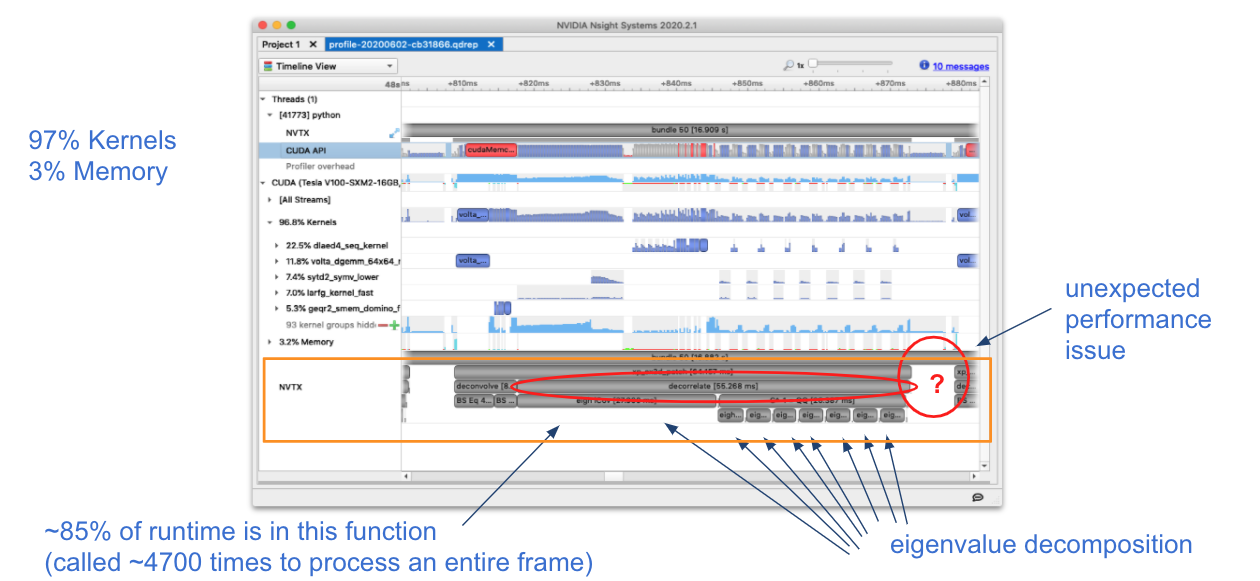
NSight Systems¶

We used NSight Systems to profile the application and identify bottlenecks in the performance. We used CUDA NVTX markers to label regions of our code using easy to identify names rather than obscure kernel names. The figure below is from an early version of our GPU port that indicated that eigenvalue decomposition operations accounted for approximately 85% of the overall runtime. Profiling also helped identify unexpected performance issues in code regions we did not expect.

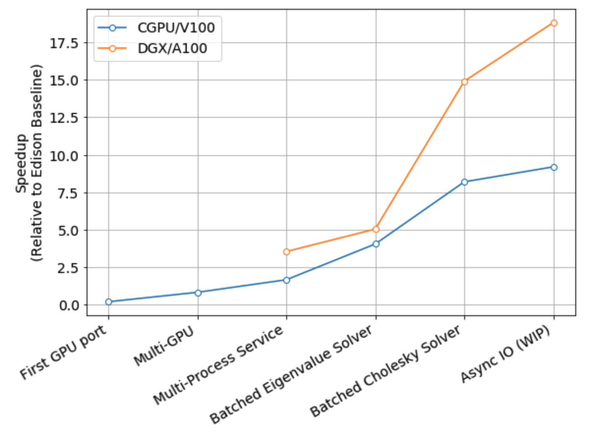
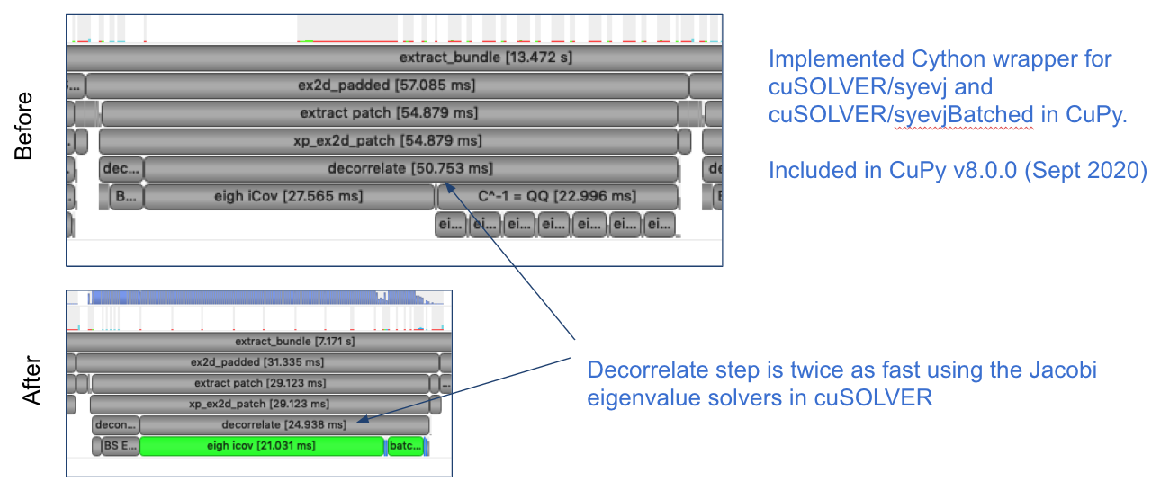
We recognized that we could "batch" the eigenvalue decomposition operations using the syevjBatched function from CUDA cuSOLVER library. This was not immediately available in Python via CuPy but we were able to implement this ourselves and contribute the functionality to CuPy.

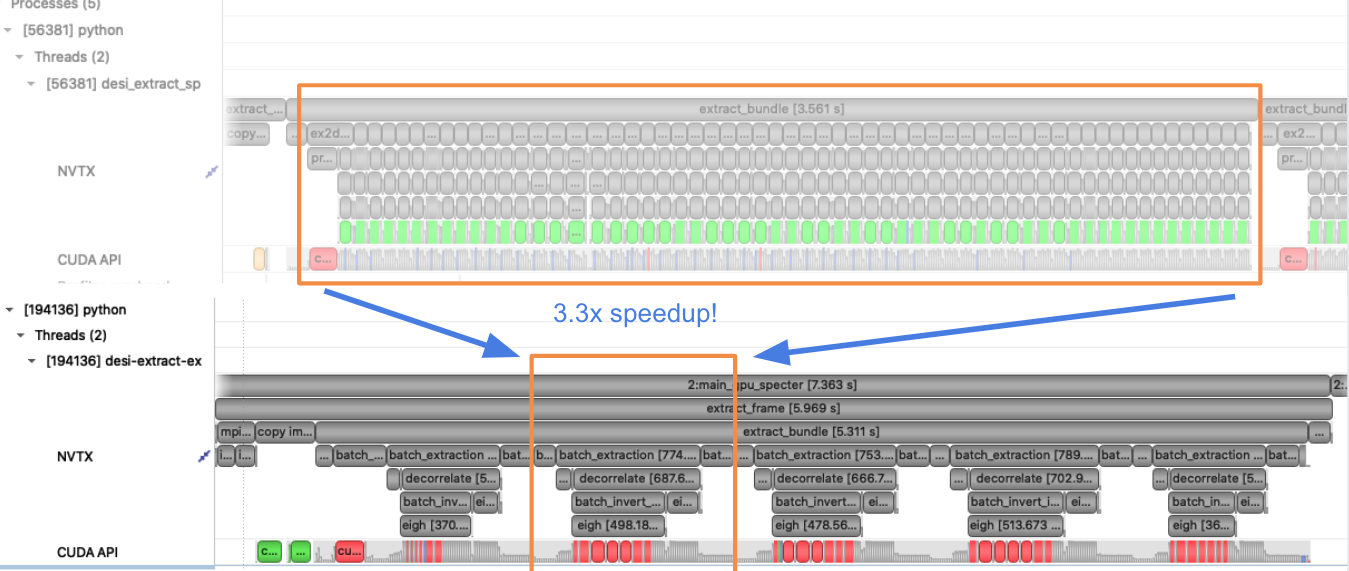
This inspired us to try batching more operations. We found a significant speedup by refactoring our problem so that we could leverage batched cholesky decomposition and solver operations (potrfBatched and potrsBatched).

MPI and CUDA Multi-Process Service¶

We use multiple GPUs in our application via MPI (mpi4py). Each rank is assigned to a single GPU. Since the CPU implementation is already using MPI, minimal refactor was required. We oversubscribe ranks to GPUs to saturate GPU utilization using CUDA Multi-Process Service (MPS), which allows kernel and memcopy operations from different processes to overlap on the GPU. We use a shell script wrapper to start the CUDA MPS process.

srun <srun args> mps-wrapper.sh app.py <app args>

Overlapping Compute and I/O¶

Reading the input image and writing the result are starting to impact the performance. After saturating GPU utilization, we were able to squeeze out more performance by putting excess CPU cores to work doing I/O. The data pipeline typically processes 30 frames from a single exposure in a single job. When there are multiple frames processed per node, the write and read steps between successive frames can be interleaved with computation. For example, after the computation group ranks have finished with frame 1, the result on the root computation rank is sent to a specially designated writer rank. The computation group ranks move on to processing the next frame which has already been read from disk by a specially designated read rank. The reader rank performs some initial preprocessing and sends the data to the root computation rank. Once the data has been sent, the reader rank begins reading the next frame. The root computation rank then broadcast the data to the rest of the computation group ranks. Meanwhile, the writer rank finishes writing the previous result and is now waiting to receive the next result.

Summary¶

Use CuPy and Numba CUDA to replace NumPy and SciPy. Saturate CPU and GPU utilization using MPI via mpi4py and CUDA Multi-Process Service. Use profiling tools like NSight Systems to identify performance bottlenecks. Offload bigger chunks of the problem to GPU using batched operations when possible. If I/O becomes an issue, try to hide it by interleaving I/O with computation using excess CPU processes.

The figure below shows the performance progress by major feature milestone.