Profiling and debugging Python¶

Here we will describe several tools and strategies for profiling Python code. These are generally in order from simplest to most complex, and we recommend that you also profile your application in a similar order.

Linaro Performance Reports for Python¶

Linaro Forge offers an easy to use profiling tool called "Performance Reports". To use this tool, you'll just need to

module load forge
perf-report srun <srun options> path/to/your/script arg1 arg2

This automatically will write .txt and .html output files which can be viewed in your text editor or browser, respectively. To view in your browser, you'll probably want to scp the data back to your local machine. No additional instrumentation or customization is required. Outputs include memory usage and MPI information. An example performance report output.

cProfile¶

Python has a nice, built-in statistical profiling module called cProfile. You can use it to collect data from your program without having to manually add any instrumentation. You can then visualize the data you collected with several tools including SnakeViz and gprof2dot.

cProfile can be used to collect data for a single process or many processes (for a Python code using mpi4py, for example.)

We will start with an example to profile a single process. In this example, we will profile a Python application at NERSC and transfer the results to our local machine to visualize. This example will generate a .prof file which contains the data we ultimately want.

Now you can run you application and collect data using cProfile:

python -m cProfile -o output.prof path/to/your/script arg1 arg2

Once your application is done running you can use scp or Globus to transfer the output.prof file to your local machine.

Now let's examine a more complex case in which we profile several processes from a Python program using mpi4py based on this page. We might want to do this to check that we are adequately load-balancing among the MPI ranks, for example. This example will write many cpu_0.prof files; one for each MPI rank. To avoid making a mess we recommend creating a new directory for your results and cd into this directory before running your application. This will also write some human-readable cpu_0.txt files (which are nice as a sanity-check but ultimately not as useful).

You will need to modify the beginning of your script by adding:

import cProfile, sys
from mpi4py.MPI import COMM_WORLD

You will also need to surround the part of your script that calls the main function with:

pr = cProfile.Profile()
pr.enable()
YOUR MAIN FUNCTION
pr.disable()

And then at the end of your program, you should add:

# Dump results:
# - for binary dump
pr.dump_stats('cpu_%d.prof' %comm.rank)
# - for text dump
with open( 'cpu_%d.txt' %comm.rank, 'w') as output_file:
    sys.stdout = output_file
    pr.print_stats( sort='time' )
    sys.stdout = sys.__stdout__

Now you can run your script as you would normally (i.e. no cProfile command is required):

python /path/to/your/script arg1 arg2

This modification will make your application write results to both a .prof file and a .txt file for each mpi rank. Then you can use scp or Globus to transfer the output files to your local machine for further analysis.

SnakeViz¶

Now that we have created a .prof file (or files) it's time to visualize the data. One browser-based option for this is SnakeViz.

We recommend that you pip install inside a conda environment. Please see the NERSC page on pip installation for more information.

You can install SnakeViz using pip:

pip install snakeviz

Then in a command line, navigate to the directory where your .prof file is located, and type:

snakeviz output.prof

This should open an interactive window in your default browser that displays the data in your .prof file. By default data are displayed in a sunburst plot:

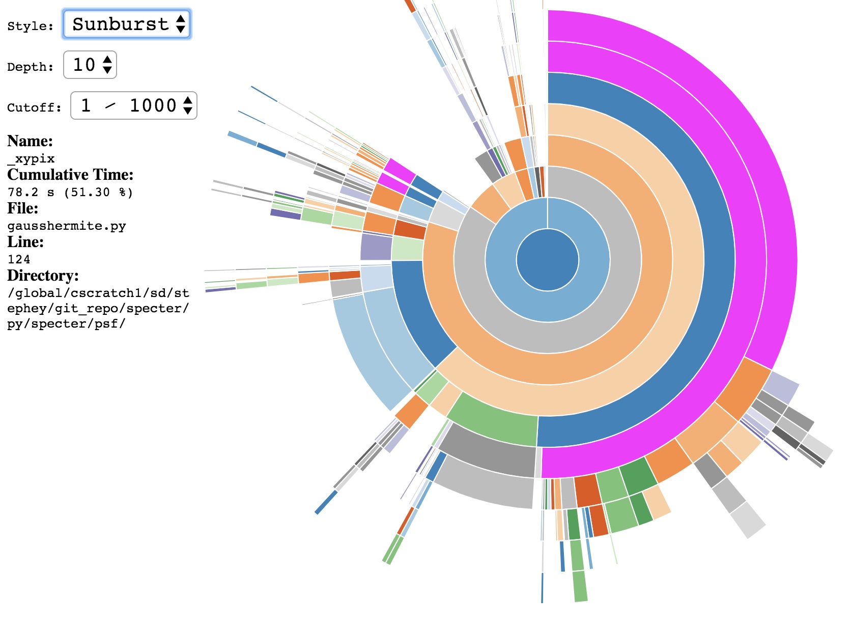
The call-stack depth can be adjusted to show deeper functions. You can also click on a particular function which will generate a new plot with the selected function now at the center.

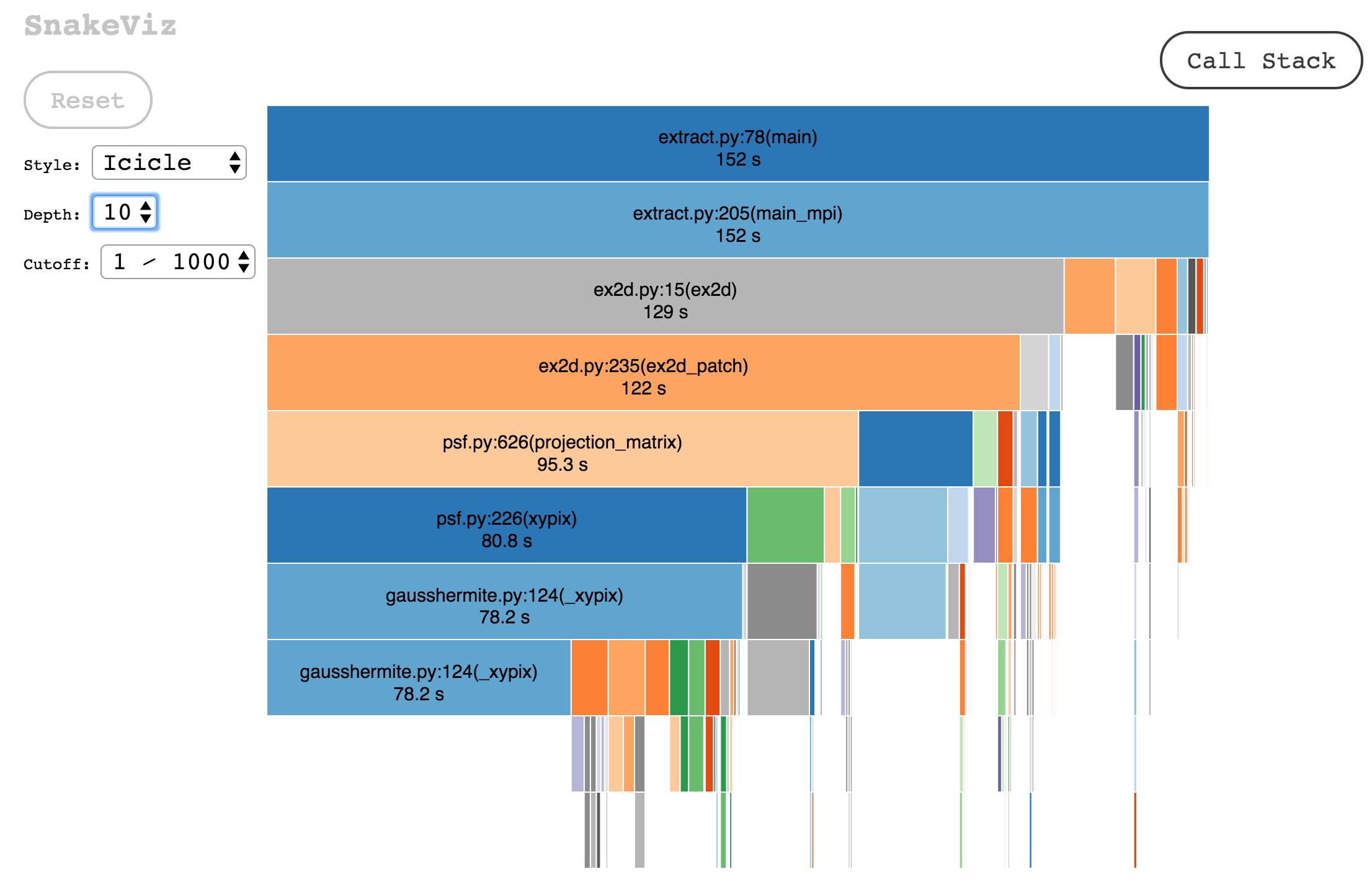
Data can also be displayed in an icicle plot:

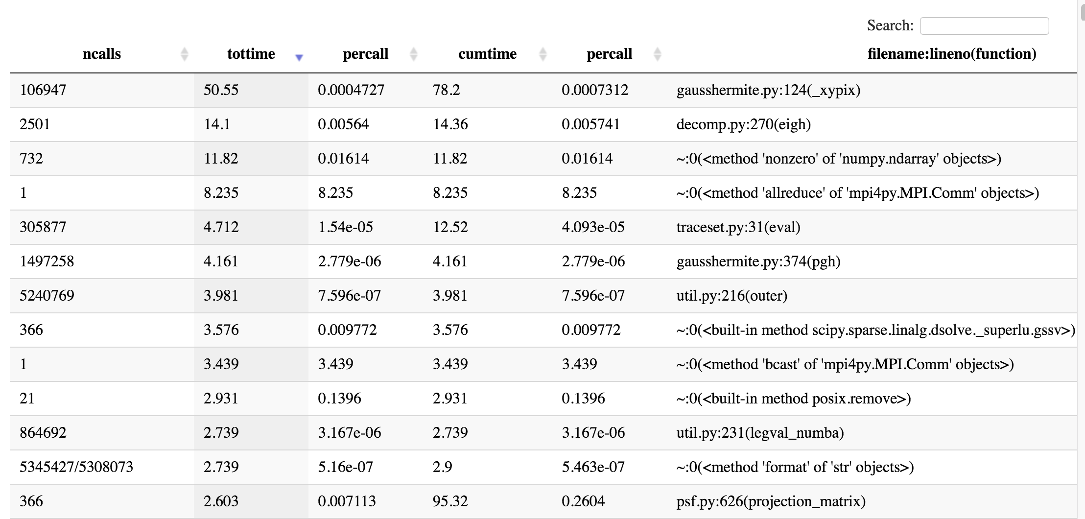
SnakeViz also creates a table listing the most expensive functions in the call-stack in descending order:

gprof2dot¶

Another option for visualizing data in a .prof file is gprof2dot. gprof2dot differs from SnakeViz in that it writes static image files (usually .png) which are perhaps easier to view and share than their browser-based cousins, but they are also not interactive.

gprof2dot displays the data in dot-graph format. Embedded in this graph is also the call-stack information. With gprof2dot it is easier to visualize the typical flow of your application than it is in SnakeViz.

Note: to use gprof2dot, you must also have graphviz installed.

You can install gprof2dot using pip install:

pip install gprof2dot

We recommend that you pip install inside a conda environment. For more information see using pip at NERSC.

Note that for gprof2dot to work correctly, you must use Python 3. Also note that you also need to either copy the gprof2dot.py file to the directory in which you will run the command, or you will need to add it to your search path through something like:

export PYTHONPATH=/path/to/where/pip/installed/gprof2dot:$PYTHONPATH

To generate the gprof2dot dot files from cProfile .prof data:

python gprof2dot.py -f pstats output.prof | dot -Tpng -o output.png

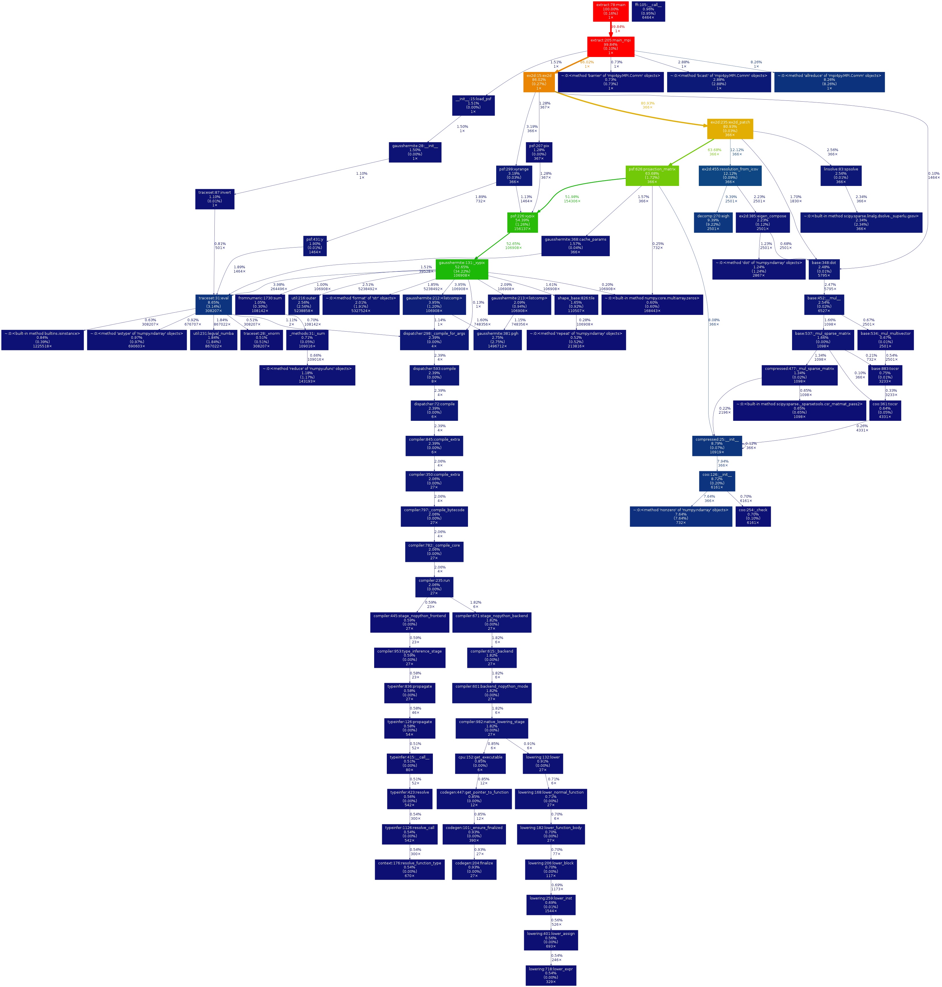
A typical gprof2dot image created from the same .prof data used in the SnakeViz section above is shown below.

If you have an MPI application and have created many .prof files, you can use shell for-loop to gprof2dot your data in a single line. Navigate to the directory in which your .prof files are located. Here is an example command to convert output from 32 MPI ranks:

for i in `seq 0 31`; do python3 gprof2dot.py -f pstats cpu_$i.prof | dot -Tpng -o cpu_$i.png; done

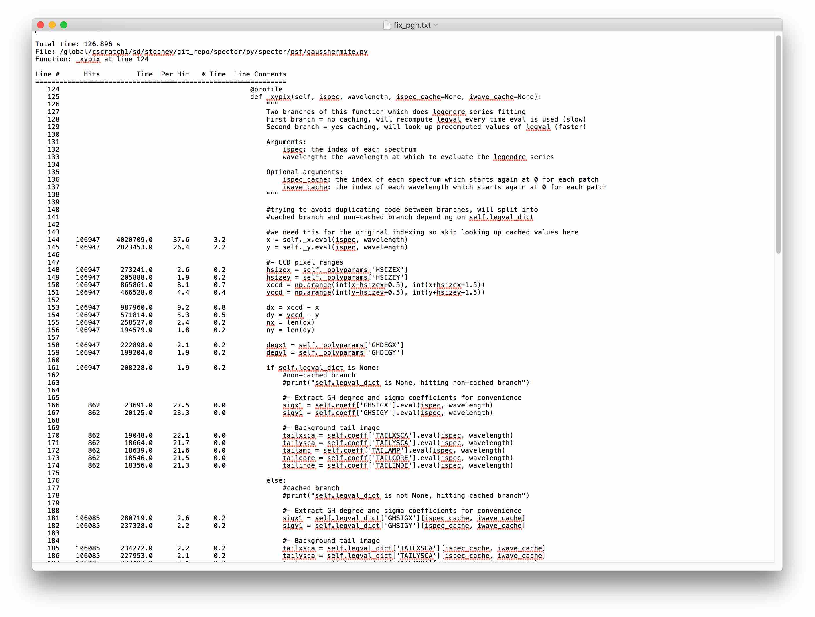
line_profiler¶

Once you have discovered where the expensive parts of your application are, it is probably time for another tool called line_profiler. This is a particularly handy tool because it gives line-by-line performance information for a selected function.

We recommend that you pip install inside a conda environment. For further reading see using pip at NERSC.

line_profiler can be installed with pip:

pip install line_profiler

Decorate the functions you want to profile with @profile.

@profile
def _xypix(arg1,arg2,arg3)
   return result

Once you have decorated the functions for which you would like line-by-line performance data, you can run line_profiler:

kernprof -l script_to_profile.py

This will write an output file with the name of your script, i.e. script_to_profile.lprof.

You'll need one more step before you get nice, human-readable output:

python -m line_profiler script_to_profile.lprof > line_profiler_out.txt

Here is the line_profiler output for our expensive function_xypix:

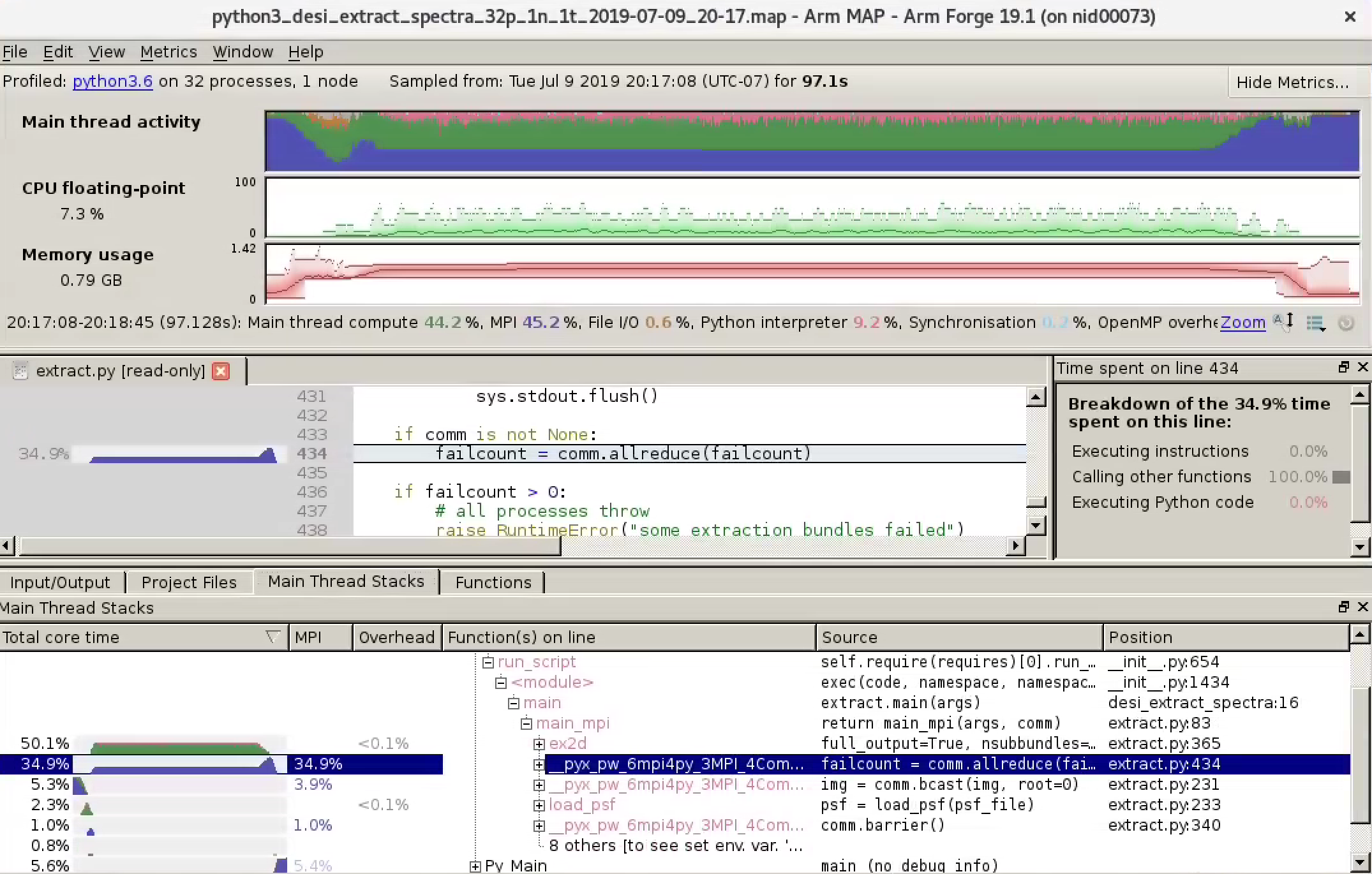
Linaro MAP for Python¶

Linaro Forge has added support for Python to their MAP profiling tool. Since this is a "big tool" we recommend that you try this tool after you have profiled your code with something simple and have some idea what you're looking for. That said, this is probably the easiest "big tool" that we support for Python on our systems. It can profile multiprocessing and single or multinode MPI jobs out of the box. Perhaps the only major drawback is that it cannot display information for individual multiprocessing threads or MPI ranks; it will only show the collected statistics for all profiled threads/ranks.

There are two ways to use MAP on our systems: either using NX or using a Remote Client/reverse connection on your own system (i.e., your laptop).

Linaro MAP using NX¶

Log onto NERSC using NX. Then, start an interactive job on a NERSC system:

salloc --account <NERSC project> --qos interactive ...

Once your interactive job starts, load the forge module and run your program with MAP:

module load forge
map python your_app.py ...

The Linaro Forge GUI window will open. Click run to start the profiling run. Don't panic: it will add some overhead to the normal runtime of your code. When the profiling data collection is finished and the statistics are aggregated, a window that displays the data from your application will automatically open. You will find the metrics displayed as a function of time, callstack information, MPI information, etc.

If you are profiling an MPI application, you will need to run: map srun python your_app.py. The difference is the srun command. One other MPI option is to use the --select-ranks option if you would like to profile only specific MPI ranks.

If you are profiling a Python multiprocessing application, you will run something like: map --no-mpi python your_app.py Unlike MPI, you will not need an srun command and adding the --no-mpi flag saves a little time (although it is not required). Note: The number of cores displayed in the top left of the MAP GUI will be incorrect. This is a known issue for Python multiprocessing that the MAP team is addressing. The rest of the profiling information should be valid, but if you notice inconsistencies, please file a ticket and we will pass your information on to the MAP team.

Linaro MAP using Remote Client¶

The workflow for using the MAP profiler from the Remote Client is similar to using NX, but with a few extra complications. The tradeoff for these additional steps is that you'll get faster response and better graphics resolution using the GUI then you would over NX.

On your local machine¶

Please check the DDT's Reverse Connect Using Remote Client section on how to download and configure the remote client.

On Perlmutter¶

After you have started the remote client, ssh to Perlmutter as you would normally. Then, start an interactive job on a NERSC system:

salloc --account <NERSC project> --qos interactive ...

Once your interactive job starts, set up your environment as necessary, load the forge module, and run your program with map --connect:

# module load python
# conda activate myenv
module load forge
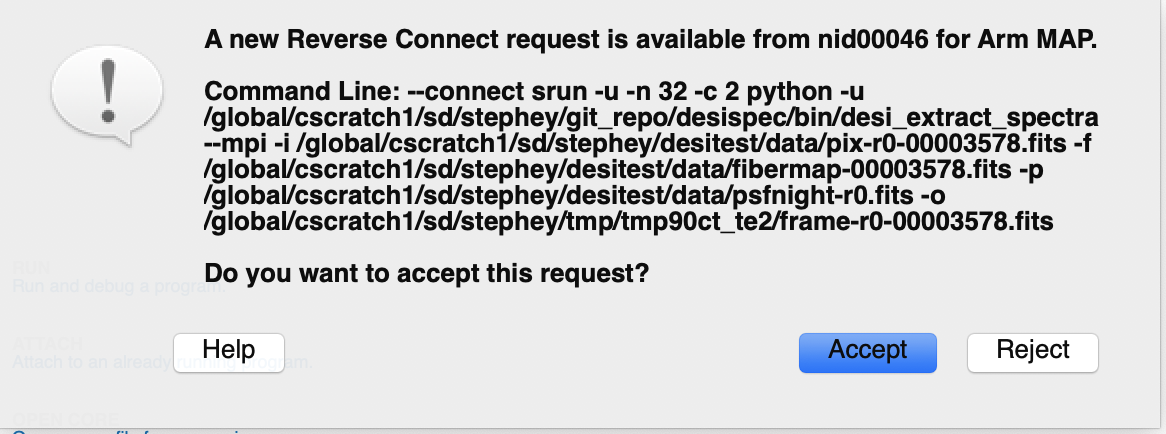
map --connect python your_app.py ...

Once you execute this command, you will be prompted to accept a reverse connection on your local machine. Click Accept and the profiling window will open and automatically start.

Once you have unchecked all but the first two CPU metrics, you can click OK and profiling will start in the same way that it did via NX. After profiling the GUI will display the results of your profiling.

Debugging Python¶

Parallel debugging can be a challenge.

Linaro Forge has released a parallel Python debugger.

To use this tool at NERSC to debug an mpi4py code:

module load forge
ddt srun -n 2 python %allinea_python_debug% hello-mpi4py.py

• Using DDT at NERSC