WRF benchmark on NERSC systems
CONUS 2.5-km
The WRF v4.4 Benchmark results. The test cases are downloaded from the NCAR MMM website: WRF v4.2.2 Benchmark Cases
The original test dataset includes a table showing example difference statistics between two identical simulations except for the compilers, which is copied below for reference:
| Variable Name | Minimum | Maximum | Average | Std Dev | Skew |
|---|---|---|---|---|---|
| U (m/s) | -0.59702 | 0.491747 | -1.77668e-07 | 0.0029298 | -0.244723 |
| V (m/s) | -0.912781 | 0.609587 | 3.43475e-07 | 0.00309517 | -0.706872 |
| W (m/s) | -0.289358 | 0.379177 | -3.34233e-08 | 0.0010013 | 1.72695 |
| T (K) | -0.550446 | 0.63913 | -4.55236e-07 | 0.00148167 | -4.40909 |
| PH (m2/s2) | -28.6036 | 30.332 | -0.000130689 | 0.0529997 | 8.22038 |
| QVAPOR (kg3/kg3) | -0.00313413 | 0.00309576 | 1.41366e-09 | 4.30677e-06 | 59.5112 |
| TSLB (K) | -0.128723 | 0.124054 | 4.4188e-07 | 0.00107553 | -0.842752 |
| MU (Pa) | -37.5372 | 38.4644 | -0.000392442 | 0.132047 | -12.7593 |
| TSK (K) | -3.11261 | 6.13058 | -9.59489e-06 | 0.0521848 | 1.32124 |
Table 1. Difference statistics across all the grid points between two simulations using an Intel vs. Gnu compilers on the NCAR Cheyenne system. PH is perturbation geopotential, QVAPOR is water vapor mixing ratio, TSLB is soil temperature, MU is perturbation dry air mass in each grid column, and TSK is skil temperature. This table is provided in the README file in the COUNS 2.5 km benchmark test.
Table 1. presents the minimum, maximum, mean, std. dev., and skewess of the difference field across grid points of the 2.5km CONUS domain. The average (middle column) is expected to be close to zero.
Perlmutter CPU nodes
Difference from the reference simulation at NCAR
The following table compares the reference simulation using an Intel compiler on the Cheynenne system at NCAR and a Perlmutter benchmark simulation using 256 MPI ranks with 4 OpenMP threads per MPI rank, compiled using the gnu environement as shown in the example build script.
| Variable Name | Minimum | Maximum | Average | Std Dev | Skew |
|---|---|---|---|---|---|
| U (m/s) | -3.00102 | 3.23068 | -1.17365e-05 | 0.0146397 | 6.05182 |
| V (m/s) | -3.75442 | 2.60446 | 2.0502e-05 | 0.013722 | 0.716138 |
| W (m/s) | -1.22846 | 1.44253 | 3.57189e-06 | 0.00493474 | 4.69308 |
| T (K) | -1.27621 | 1.57364 | 0.000151034 | 0.00725031 | -3.66369 |
| PH (m2/s2) | -41.4504 | 31.1257 | 0.0641135 | 0.277627 | 0.227528 |
| QVAPOR (kg3/kg3) | -0.00293566 | 0.00332439 | -1.42891e-08 | 5.01009e-06 | 81.573 |
| TSLB (K) | -0.192291 | 0.107086 | 0.000112013 | 0.00209734 | -17.2706 |
| MU (Pa) | -38.5956 | 36.2664 | -0.0229563 | 0.363282 | 1.91311 |
| TSK (K) | -6.19937 | 3.93146 | 0.0107928 | 0.0681577 | 2.56526 |
Table 2. Difference statistics between the reference simulation using an Intel compiler on the NCAR Cheyenne system vs. a benchmark run on Perlmutter compiled by the gnu compiler.
Compared to Table 1., the difference statistics are larger in Table 2 by an order of magnitude. Still, the domain-average differences are close to zero for all the variables, indicating that the WRF simulation on Perlmutter is statistically indistinguishable from the reference simulation run by the WRF development team at NCAR.
Benchmark on Perlmutter

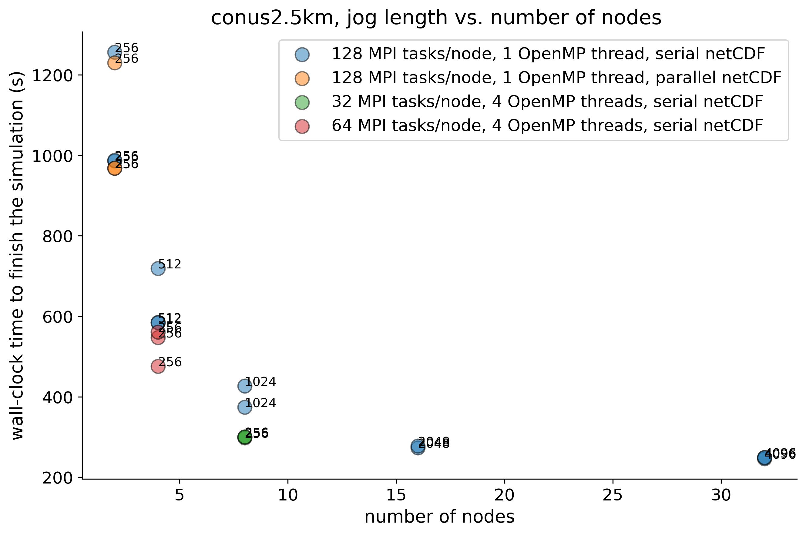
Figure 1. Weak scaling of the CONUS 2.5-km case on Perlmutter. Numbers next to the markers are the number of MPI tasks.
Figure 1. shows the benchmark test of the CONUS 2.5-km case on Perlmutter. Main points are:
-
WRF simulation becomes exponentially faster as the number of nodes (MPI ranks) are increased to ~16 nodes or 2048 MPI ranks (880 grid columns per MPI rank). Larger resource use does not seem to provide much more advantage.
-
8 nodes with 256 MPI ranks and 4 OpenMP threads per MPI rank is nearly as fast as the 16-node job, with a half of the simulation cost compared to the 16-node job.
-
Parallel netcdf option with "stripe_small" set for the output directory (see Lustre file striping) shortens the time spent on writing the output file from 20-40 seconds to 3-5 seconds. This difference is not visible in the graph because the testcase writes out only one history file after the one-hour integration. If, however, we write 6 history files at 10-minutes interval, then the difference between serial and parallel netcdf I/O would be ~ 180 seconds vs. 24 seconds per one hour integration. For 24-hour model integration, then the difference would be 4320 seconds (1.2 hours spent on writing outputs) vs. 576 seconds (~10 minutes spent on writing output).